PAULA: A Computational Substrate for Self-Organizing Biologically-Plausible AI
Introducing a novel, biologically-grounded neural architecture that achieves self-organizing representation and temporal dimensionality expansion. By leveraging purely local learning rules and homeostatic metaplasticity, PAULA demonstrates that robust, adaptive computation can emerge naturally—without the need for global backpropagation.
Abstract
Modern Artificial Neural Networks (ANNs), despite their successes, diverge significantly from biological neural computation. They rely on static functions where learning occurs through global backpropagation rather than continuous local adaptation. We introduce PAULA (Predictive Adaptive Unsupervised Learning Agent), a biologically inspired neuron model incorporating: predictive coding for local error dynamics, retrograde modulation of vector-based synapses, and a homeostatic metaplasticity mechanism that adapts learning windows and thresholds to maintain bounded activity.
Using an in silico pipeline, we validate this model on MNIST. The architecture cleanly separates representation from readout: PAULA produces temporally structured dynamical states, while an independently trained SNN decoder reads those states—analogous to how EEG and fMRI read neural activity without producing it. Results demonstrate substantial computational power even at the single-unit level (38.1% accuracy from one neuron) and reveal emergent network properties including graceful degradation under damage, superior performance with sparse architectures (86.8% decoder accuracy), and spontaneous self-organization of functional cell assemblies.
Ablation studies reveal the system implements temporal dimensionality expansion through variance-driven self-organization, with complex temporal patterns collapsing 25% when multi-scale integration is prevented. This validates PAULA as a substrate for developing robust, adaptive AI through biologically-grounded self-organizing mechanisms.
Key Findings
PAULA demonstrates substantial computational capabilities even at the single-unit level: a single neuron with adaptive dynamics achieves 38.1% on MNIST (nearly 4 times the random chance), demonstrating that temporal dynamics and homeostatic metaplasticity carry significant computational power. Full 25%-sparse networks produce representations that an external SNN decoder reads at 86.8% accuracy, relying entirely on local, unsupervised learning.
The core innovation is temporal dimensionality expansion through self-organizing multi-scale projection. Ablation studies validate this mechanism: complex temporal patterns collapse by 25% when multi-scale integration is removed, while simple patterns remain virtually unaffected.
A sparsity law emerges where 25% connectivity outperforms 100% dense networks by over 8 percentage points. Sparse networks converge to stable solutions noticeably better than dense networks, which fail to stabilize in reasonable time. Throughout training, functional cell assemblies self-organize without any supervisory signal.
1. Introduction: Why a New Approach?
In traditional artificial neural networks, a neuron is a static mathematical function: it takes inputs, applies weights, sums them up, and passes the result through an activation function. A biological neuron, however, is something far more complex: a dynamic, adaptive agent that learns from purely local information and continuously adjusts to its environment (Moore et al., 2024; Liu et al., 2025; Patel et al., 2025). This biological premise forms the foundation of the ALERM framework (Architecture, Learning, Energy, Recall, and Memory), for which PAULA serves as the primary empirical validation.
This divergence suggests that current AI is solving the wrong problem (Chen et al., 2025). Rather than merely approximating static functions (input/output mappings), biological intelligence is fundamentally about constructing and maintaining dynamical states that mirror environmental structure.
"Intelligence is not programmed; it emerges through continuous interaction with an environment. Any persistent system must model its environment to survive."
- Derived from Karl Friston's Free Energy Principle
Biological neural networks operate under fundamentally different principles:
- Local Learning: Neurons learn through local synaptic plasticity without global error signals
- Homeostatic Regulation: They maintain stability through self-regulation (Niemeyer et al., 2022; Shen et al., 2024)
- Metaplasticity: They adapt their learning rates based on activity history (Kuśmierz et al., 2017)
A fundamental challenge in temporal pattern learning is the temporal ambiguity problem: different temporal sequences can appear identical when compressed into static representations. Consider handwritten digit recognition: digit 8 (top loop → connector → bottom loop) and digit 0 (single loop) can look similar in static images, yet their temporal production differs substantially. Standard neural networks struggle with such distinctions because they lack explicit temporal representation.
We frame this as a dimensionality expansion problem: to disentangle temporally ambiguous patterns, a system must project low-dimensional signals into high-dimensional representations where patterns become linearly separable. This is analogous to the kernel trick in classical machine learning, where input data is implicitly mapped to higher dimensions to enable linear classification. However, in the temporal domain, this expansion must be self-organizing: adapting to signal statistics without explicit design.
This paper makes three contributions:
- A self-organizing temporal dimensionality expansion mechanism that amplifies temporal variance through multiplicative weight dynamics and projects signals into multi-scale representations through adaptive metaplasticity.
- Empirical validation of mechanism necessity showing that complex temporal patterns collapse by 25% when multi-scale integration is prevented, while simple patterns remain unaffected, proving that expansion adapts to signal complexity.
- Integration with recent advances in homeostatic plasticity and three-factor learning, positioning the work within the emerging convergence on energy-efficient predictive coding in spiking neural networks.
We developed PAULA to realize these contributions through a novel formal model for a network of dynamic, self-regulating computational units that learn continuously based on principles of local prediction (N'dri et al., 2025). This model synthesizes a wide range of neuroscientific discoveries into a single, coherent mathematical framework.
Central Theoretical Claim
Beyond the empirical results, PAULA's most original contribution is a hypothesis about the nature of representation itself: representation is not a static pattern stored in weights; it is a process. Memory is an attractor landscape; recognition is re-enactment of a learned dynamical regime. This processual representation hypothesis (§7.2) reframes what it means for a neural system to "know" something, with implications for memory, forgetting, and meta-cognition.
2. The PAULA Model
At its core, PAULA defines a "smart neuron": a biologically-inspired computational unit that goes beyond traditional artificial neural network primitives. In this section, we present a comprehensive specification of the model's architecture.
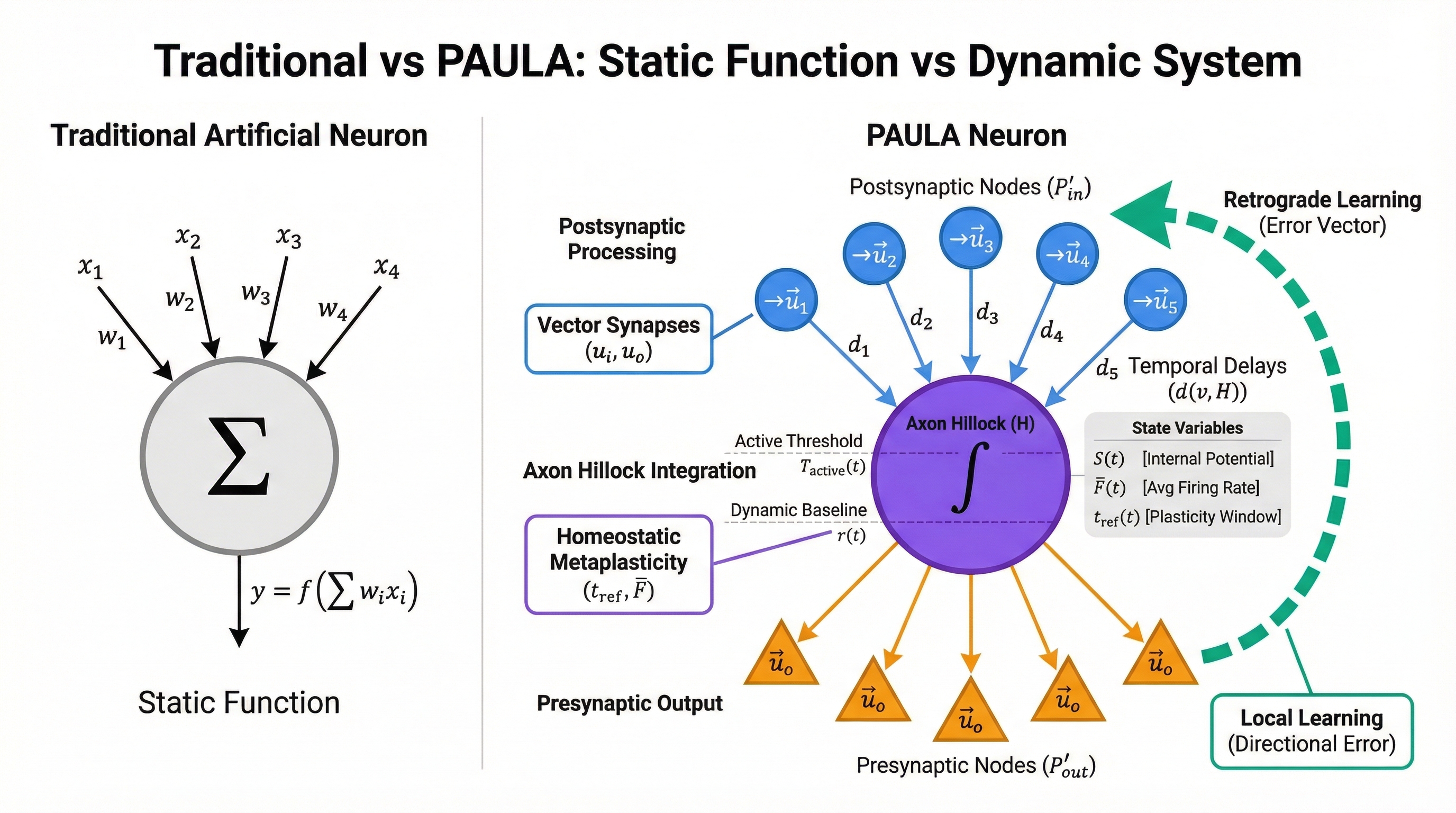
2.1 Graph Architecture
We formally define each neuron as a weighted, directed graph \(G = (V, E, d)\), where:
-
Node Sets: The node set \(V\) is the union of
three distinct processing sets:
- \(V_{P'_{in}}\): The set of all postsynaptic processing nodes
- \(V_{P'_{out}}\): The set of all presynaptic processing nodes
- \(\{H\}\): The axon hillock node
- Complete Node Set: \(V = V_{P'_{in}} \cup \{H\} \cup V_{P'_{out}}\)
- Edges: \(E \subseteq V \times V\) represents the directed connections between nodes
- Weights: A distance function \(d: E \to \mathbb{N}\) that assigns a travel time (in ticks) to each edge
2.2 Fundamental Units
-
Input Unit (\(i\)): A postsynaptic receptor. The
\(I_{adapt}\) set is a family of abstract functional subtypes:
- \(I_{adapt, Excitability}\)
- \(I_{adapt, Metaplasticity}\)
-
Output Unit (\(o\)): A presynaptic
neurotransmitter release. The \(O_{mod}\) set includes:
- \(O_{mod, Excitability}\)
- \(O_{mod, Metaplasticity}\)
2.3 Integrated Interaction Points (\(P′\))
Postsynaptic Point (\(P'_{in}\)): Its state is defined by a vector of receptor efficacies. Each synapse maintains multiple distinct strengths: one for information flow and others for adapting to excitability and metaplasticity signals:
\[\vec{u_i} = (u_{info}, u_{adapt, Excitability}, u_{adapt, Metaplasticity}, ...)\]
Presynaptic Point (\(P'_{out}\)): Its output vector includes corresponding neuromodulator types. When a neuron fires, it releases signals that carry information and also modulate the behavior of the receiving neurons:
\[\vec{u_o} = (u_{info}, u_{mod, Excitability}, u_{mod, Metaplasticity}, ...)\]
2.4 System State Variables and Parameters
Tick-Dependent Variables:
- \(S(t)\): Internal potential at the axon hillock \(H\)
- \(O(t)\): Output signal function from the hillock \(H\)
- \(t_{last\_fire}\): Timestamp of the last somatic firing event
- \(\bar{F}(t)\): The long-term average firing rate
- \(\vec{M}(t)\): The neuromodulatory state vector (\(\vec{M}(t) = (M_{Excitability}(t), M_{Metaplasticity}(t), ...)\))
- \(r(t), b(t)\): The dynamic primary and post-cooldown thresholds
- \(t_{ref}(t)\): The plastic causal time window for learning
Constant Parameters:
- \(\delta_{decay}\): Per-tick potential decay factor
- \(\beta_{avg}\): Decay factor for the average firing rate EMA
- \(\eta_{post}\): The postsynaptic learning rate
- \(\eta_{retro}\): The presynaptic learning rate for retrograde adaptation
- \(c\): The activation cooldown period in ticks
- \(\lambda\): The membrane time constant for the axon hillock
- \(p\): The constant magnitude of every output signal
- \(r_{base}, b_{base}\): Baseline values for the dynamic thresholds
- \(\vec{\gamma}\): Vector of decay factors for each component of \(\vec{M}(t)\)
- \(\vec{w}_r, \vec{w}_b, \vec{w}_{tref}\): Sensitivity vectors for dynamic parameters
2.5 State Transitions (The "Tick" and Graph-Based Dynamics)
The system evolves over discrete time steps \(dt\).
A. Neuromodulation and Dynamic Parameter Update:
-
Aggregate Neuromodulatory Input: For each
modulator type \(k\), calculate the total weighted input signal.
This sums up all the external "control signals" (like excitability
and metaplasticity) arriving at each synapse, weighted by how
sensitive that synapse is to each type:
\[\text{total\_adapt\_signal}_{k}(t) = \sum_{v \in V_{P'_{in}}} \left( O_{ext, mod, k}^{(v)}(t) \cdot u_{i, adapt, k}^{(v)}(t) \right)\]
-
Update Neuromodulatory State Vector: The internal
"state of mind" of the neuron updates as an exponential moving
average; it slowly forgets past modulation while incorporating new
signals:
\[M_k(t+dt) = \gamma_k \cdot M_k(t) + (1-\gamma_k) \cdot \text{total\_adapt\_signal}_k(t)\]
-
Update Average Firing Rate: The neuron tracks how
often it fires over time. This running average is key for
homeostasis: it lets the neuron notice if it is too active or too
quiet:
\[\bar{F}(t+dt) = \beta_{avg} \cdot \bar{F}(t) + (1-\beta_{avg}) \cdot O(t)\]
-
Calculate Final Dynamic Parameters: These
equations set the firing thresholds of the neuron based on its
neuromodulatory state. The thresholds \(r\) and \(b\) shift up or
down depending on the accumulated modulation:
\[\begin{align*} r(t+dt) &= r_{base} + \vec{w}_r \cdot \vec{M}(t+dt) \\ b(t+dt) &= b_{base} + \vec{w}_b \cdot \vec{M}(t+dt) \end{align*}\]
Adaptive Refractory Period (Multi-Scale Projection): The plasticity window \(t_{ref}\) creates heterogeneous temporal integration windows that enable multi-scale projection:
\[\begin{align*} t_{ref\_homeostatic}(t) &= \text{upper\_bound} - (\text{upper\_bound} - \text{lower\_bound}) \cdot (\bar{F}(t) \cdot c) \\ t_{ref}(t+dt) &= t_{ref\_homeostatic}(t) + \vec{w}_{tref} \cdot \vec{M}(t+dt) \end{align*}\]
Mechanism: High-firing neurons (large weights, high variance) → short \(t_{ref}\) (~90 ticks). Low-firing neurons (small weights, low variance) → long \(t_{ref}\) (~150 ticks).
Function: Different neurons become selective to different temporal scales. Short windows capture fast transitions (e.g., connector strokes in digit 8), while long windows maintain global context (e.g., full loop structure). Together, they project input into high-dimensional multi-scale representations. This provides the projection mechanism itself.
B. Input Processing & Propagation:
When a signal arrives at a synapse, it gets multiplied by the strength of that synapse: this is how learning shapes perception:
-
When an external signal vector \(\vec{O}_{ext}\) arrives at a node
\(v \in V_{P'_{in}}\), the local voltage is computed as the signal
times the synaptic weight:
\[V_{local}(t) = O_{ext, info} \cdot u_{info}^{(v)}(t)\]
- This \(V_{local}\) potential is scheduled for arrival at the axon hillock \(H\) at \(t_{arrival} = t + d(v, H)\). The delay models realistic signal propagation time along the dendrite.
C. Signal Integration at Axon Hillock:
All incoming signals are summed at the cell body, but each is weakened by how far it had to travel (longer paths = more decay):
\[I(t) = \sum V_{local}(t) \cdot (\delta_{decay})^{d(v, H)}\]
D. Somatic Firing:
The core spiking dynamics. The membrane potential rises toward input and decays toward rest, like a leaky bucket:
-
State Evolution: The membrane potential \(S\)
evolves as a leaky integrator; it accumulates input while
constantly draining toward zero:
\[S(t+dt) = S(t) + \frac{dt}{\lambda} (-S(t) + I(t))\]
- Firing Condition: A spike occurs if \(S(t+dt) \ge T_{active}(t)\) and \(t+dt \ge t_{last\_fire} + c\). The neuron must exceed threshold AND wait out its refractory cooldown.
- Instantaneous Firing Dynamics: If a spike occurs at \(t_{fire}\), apply axon hillock reset rules (membrane resets, threshold jumps up to prevent immediate re-firing).
- Threshold Reset: If \(S(t)\) decays to near-zero, \(T_{active}(t)\) resets to \(r(t)\). This prepares the neuron for the next cycle of input.
E. Output and Learning:
- Presynaptic Release: A somatic spike propagates to all \(v \in V_{P'_{out}}\), causing release of \(\vec{u_o}^{(v)}\)
-
Dendritic Computation & Plasticity: At a synapse
\(v \in V_{P'_{in}}\) receiving \(\vec{O}_{ext}\):
-
Step 1: Directional Error Calculation: The
mismatch between what the synapse expected (its weight) and
what actually arrived. This local error drives learning:
\[\vec{E}_{dir}(t) = \vec{O}_{ext}(t) - \vec{u_i}^{(v)}(t)\]
-
Step 2: Temporal Correlation (Plasticity Gating)
: The key STDP-like mechanism. If the input arrived within the
plasticity window after the neuron fired, strengthen the
connection ("neurons that fire together, wire together"). If
too late, weaken it:
- Calculate \(\Delta t = t - t_{last\_fire}\) (time since last spike)
- If \(\Delta t \le t_{ref}(t)\), set direction = +1 (LTP: long-term potentiation)
- If \(\Delta t > t_{ref}(t)\), set direction = -1 (LTD: long-term depression)
-
Step 3: Postsynaptic Update: The actual
learning: adjust the synaptic weight proportionally to the
error magnitude, the current weight (multiplicative update),
and the temporal direction (LTP vs LTD):
\[\Delta u_{info}^{(v)}(t+dt) = \eta_{post} \cdot \text{direction} \cdot ||{E}_{dir}(t)|| \cdot u_{info}^{(v)}(t)\]
Variance Amplification: This multiplicative form creates intentional variance amplification. Large weights receive larger updates, causing neurons to diverge in their firing rates. High-firing neurons (processing high-variance temporal patterns) develop distinct properties from low-firing neurons, creating the heterogeneity necessary for multi-scale processing.
-
Step 4: Retrograde Signal and Presynaptic Update
: The postsynaptic neuron sends a directed error signal back
to the presynaptic neuron, allowing bilateral learning without
global supervision. The upstream neuron adjusts its output
accordingly:
\[\begin{align*} \vec{O}_{retro}(t) &= \text{direction} \cdot \vec{E}_{dir}(t) \\ \Delta \vec{u_o}(t+dt) &= \eta_{retro} \cdot \vec{O}_{retro}(t) \end{align*}\]
-
Step 1: Directional Error Calculation: The
mismatch between what the synapse expected (its weight) and
what actually arrived. This local error drives learning:
3. Experimental Methodology
Testing a new neuron model like PAULA required a carefully designed experimental setup. We could not simply train it like a regular neural network. We needed to create an entire research pipeline that treats the PAULA network as a living system we can observe, measure, and understand.
3.1 Network Construction
We built deep perceptron-style networks made entirely of PAULA neurons. These are fully-connected layers where each neuron connects to every neuron in the next layer, but we systematically varied the connection density to see how sparsity affects learning and performance.
Each network was designed as a directed graph: neurons as nodes, synapses as edges with propagation delays. The interactive builder let us experiment with different layer sizes, depths, and connection patterns to find the sweet spot for biological plausibility and computational power.
Code: Network Builder
Interactive tool for designing PAULA networks with real-time visualization
code View Source3.2 Activity Recording
We fed MNIST images to the networks one by one, recording everything that happened inside the network during processing, not just the final answer.
For each image, we captured: membrane potentials (how excited each neuron was over time), plasticity windows (the dynamic learning sensitivity), neuromodulatory signals (internal control mechanisms), and spike timing (exact moments when neurons fired). This gave us a complete temporal fingerprint of how the network "thought" about each digit.
Code: Activity Recorder
Simulates network response to image sequences and logs all internal dynamics
code View Source3.3 Preparing Data for Analysis
Raw activity logs are messy, containing gigabytes of temporal data per network. We needed to extract meaningful features that a classifier could learn from. We focused on the key dynamical signatures: average membrane potentials over time, firing rates, and temporal patterns in the plasticity parameters.
This transformed the network's continuous internal dynamics into structured datasets that could be fed into standard machine learning pipelines for analysis and evaluation.
Code: Data Processor
Converts raw activity logs into PyTorch datasets with temporal feature extraction
code View Source3.4 Training the Pattern Decoder
To measure what the PAULA network actually learned, we trained an external spiking neural network classifier to decode the activity patterns. This serves as an "EEG" device that reads brain activity and translates it into recognizable categories.
The classifier used a simple but effective architecture: input layer for the extracted features, a couple of hidden layers with leaky integrate-and-fire neurons, and an output layer that predicts digit classes. We trained it using standard techniques: cross-entropy loss, Adam optimizer, and a learning rate of 0.0005. The extracted features were genuine signatures of neural computation that happened inside PAULA units.
Code: Pattern Decoder
Trains SNN classifier to decode PAULA network activity patterns into digit predictions
code View Source3.5 Real-Time Evaluation
Final evaluation went beyond simple accuracy metrics. We ran the networks in real-time, watching how their "thinking" evolved over time. Some networks made quick decisions, others took longer to deliberate, revealing cognitive dynamics that static classifiers would miss.
The "thinking mode" experiments were particularly revealing: by giving networks extra processing time, we could see which digits required fast recognition versus deep deliberation, mirroring how humans process familiar versus complex stimuli.
Code: Live Evaluator
Real-time performance testing with temporal analysis and extended processing capabilities
code View Source3.6 Evaluation Protocol
To ensure comprehensive and reproducible results, we established a systematic evaluation protocol across all experiments. Every network architecture was evaluated under five distinct "thinking mode" configurations, where the network is given varying amounts of processing time (measured in simulation ticks) to integrate evidence:
- No thinking mode: Standard processing with base time allocation
- Thinking ×2: Extended processing time at 2× base duration
- Thinking ×3: Extended processing time at 3× base duration
- Thinking ×5: Extended processing time at 5× base duration
- Thinking ×7: Extended processing time at 7× base duration
This evaluation matrix was applied consistently across three distinct network architectures (single neuron, sparse networks, and dense networks), yielding 15 unique experimental conditions. All results reported in this paper are drawn from this comprehensive evaluation set, ensuring that observed phenomena are robust across different temporal integration scales and architectural configurations.
3.7 Structural Analysis
A significant insight came from analyzing what emerged inside the networks during learning. We used clustering algorithms to find functional groups of neurons that specialized in different aspects of the task, dynamical systems analysis to map the network's behavioral landscape, and performance analysis to understand scaling relationships.
This multi-modal approach revealed that PAULA networks self-organize into sophisticated computational architectures that mirror biological neural systems.
Analysis Tools
Scripts for analyzing emergent network properties and visualization
4. Key Results
4.1 Single Neuron Computational Power
Our first experiments aimed to establish the computational capacity of a single PAULA neuron. The relevant control is random chance (10% for 10-class classification). A single adaptive neuron with homeostatic metaplasticity achieves remarkable performance on MNIST, far exceeding chance, demonstrating that the adaptive dynamics (not the parameter count) are doing the work. This supports the view that single neurons represent powerful computational units capable of solving complex tasks (Jones & Kording, 2020).
Analysis of the neuron's temporal dynamics reveals that it encodes digit identity through characteristic membrane potential trajectories rather than static response magnitudes. Different digits produce different temporal patterns in the integrated response, with the external decoder learning to read these trajectories. This demonstrates that computational richness emerges from temporal dynamics and adaptive mechanisms, not from parameter counts, validating the hypothesis that neurons are dynamical systems rather than static functions.
Result 1: The "Impossible" Test
A network consisting of a single neuron was tasked with classifying all 10 MNIST digits. The final, optimized result achieved a Top-1 accuracy of 24.1% compared to the random baseline of 10%.
Result 2: Single-Neuron Cognition
Applying "thinking mode" (granting additional processing time) pushed the Top-1 accuracy to 38.1%. Analysis revealed a distinct cognitive profile: the neuron showed "fast" recognition for simple digits ('0', '1') and "deliberative" recognition for complex temporal patterns (improving '5' from 0% to 71% Top-3 accuracy with extra time).
Single Neuron Performance with Extended Processing Time
| Condition | Top-1 Accuracy | Top-3 Accuracy |
|---|---|---|
| No thinking | 24.1% | 53.6% |
| Thinking ×2 | 31.3% | 51.8% |
| Thinking ×3 | 35.6% | 55.5% |
| Thinking ×5 | 37.5% | 53.5% |
| Thinking ×7 | 38.1% | 53.5% |
Beyond classification accuracy, the single neuron demonstrates remarkable dimensionality reduction: compressing 784-dimensional input into a 2-dimensional dynamical state (⟨S⟩, ⟨t_ref⟩) while preserving ~40% of class-discriminative information.
4.2 Systemic Properties & Architectural Principles
Next, we tested the behavior of multi-neuron networks, uncovering key design principles that emerge from PAULA's local learning dynamics.
Result 3: Graceful Degradation
When trained and tested on a dataset corrupted with a "state bleed" bug (temporal noise due to not reinitializing the network between different samples of the same digit label), the system's performance did not collapse. It maintained ~45% accuracy, demonstrating inherent robustness and resilience, a hallmark of biological systems.
Result 4: The Sparsity Scaling Law
A controlled experiment on networks with 144 neurons revealed a clear inverse correlation between connectivity and baseline performance:
- 100% Density: 64.2% Top-1 Accuracy
- 50% Density: 70.6% Top-1 Accuracy
- 25% Density: 76.1% Top-1 Accuracy
Result 5: The Architectural "Sweet Spot"
The best-performing model across all experiments was a smaller, 80-neuron sparse network, which achieved a Top-1 accuracy of 81.3%. Notably, bigger is not better: performance is a function of intelligent architecture (layer structure, neuron count, sparsity) rather than sheer scale; another key biological principle.
Detailed Performance Metrics
| Density | Best Top-1 | Best Top-3 | Best Time | Avg Ticks to Correct | Prediction Stability |
|---|---|---|---|---|---|
| 25% | 86.80% | 94.20% | 79 | 31.02 | 96.88% |
| 50% | 81.80% | 94.30% | 95 | 29.22 | 95.01% |
| 100% | 78.60% | 92.40% | 140 | 36.18 | 92.47% |
Network sparsity critically influences homeostatic dynamics and performance. The 25% sparse network achieves 86.8% accuracy, outperforming both 50% sparse (80.9% Top-1 base accuracy) and 100% dense (78.6% Top-1 base accuracy) configurations. Analysis of homeostatic parameters reveals the mechanism: dense networks show Layer 1 saturation, with neurons clustered at the \(t_{ref}\) lower bound (88-90), while sparse networks maintain better \(t_{ref}\) diversity (88-96). This pattern indicates that full connectivity creates excessive input drive, pushing all neurons toward maximal selectivity and hurting the heterogeneity necessary for specialization. Sparse connectivity, by contrast, allows neurons to operate across expanded homeostatic range, enabling differentiated responses and emergent cell assemblies.
Comparison with Existing Paradigms
To contextualize these results, we compared the PAULA architecture against leading biologically-plausible models and standard ANNs on the MNIST task. The comparison dimension here is learning paradigm, not absolute accuracy: PAULA operates under fundamentally different constraints. It uses 6× less training data (10k vs. 60k samples), learns through purely local, unsupervised, gradient-free rules with no global error signal, and requires no labeled data during representation learning. Labels are only used by the external SNN decoder.
| Model | Objective / Paradigm | Optimization Math | Local Error Signal | Restricted Data | Accuracy |
|---|---|---|---|---|---|
| Standard ANN | Global Supervised | Backpropagation | None | No (60k) | ~99% |
| DECOLLE | Local Supervised | Surrogate Gradients | Auxiliary Classifier | No (60k) | ~98% |
| STDP-CNN | Unsupervised | Hebbian / STDP | None | No (60k) | ~98% |
| PAULA (Sparse) | Unsupervised / ALERM | Gradient-Free | Predictive Coding | Yes (10k) | 86.8% |
| PAULA (CNN) | Unsupervised / ALERM | Gradient-Free | Predictive Coding | Yes (10k) | 96.55% |
4.3 "Thinking Mode" and Temporal Integration
To further characterize the network's cognitive dynamics, we applied extended processing time, what we call "thinking mode", to the best-performing sparse network:
⏱️ Temporal Evidence Integration
- Final Performance: 86.8% Top-1, 93.9% Top-3 accuracy
- Thinking Bonus: +15.2% absolute improvement
- Hypothesis Formation: Correct answer appears in Top-3 at ~16.8 ticks
- Deliberation & Confirmation: Final correct Top-1 decision at ~24.9 ticks
The model is not a static classifier. It is a dynamic decision-making engine that demonstrably integrates evidence over time, mirroring cognitive models like the Drift-Diffusion Model.
4.4 Emergent Cell Assemblies
Our clustering analysis, analogous to fMRI in neuroscience, revealed that PAULA networks spontaneously self-organize into 4-6 distinct functional "cell assemblies". These are groups of neurons that encode similar features:
Interactive Neuron Cluster Visualizations (hover for details, click+drag to zoom)
This emergent organization mirrors biological cortical columns, where neurons spanning multiple layers form functional units based on shared response properties. Critically, PAULA produces this organization without explicit architectural constraints or supervised grouping. It arises purely from homeostatic regulation interacting with task statistics.
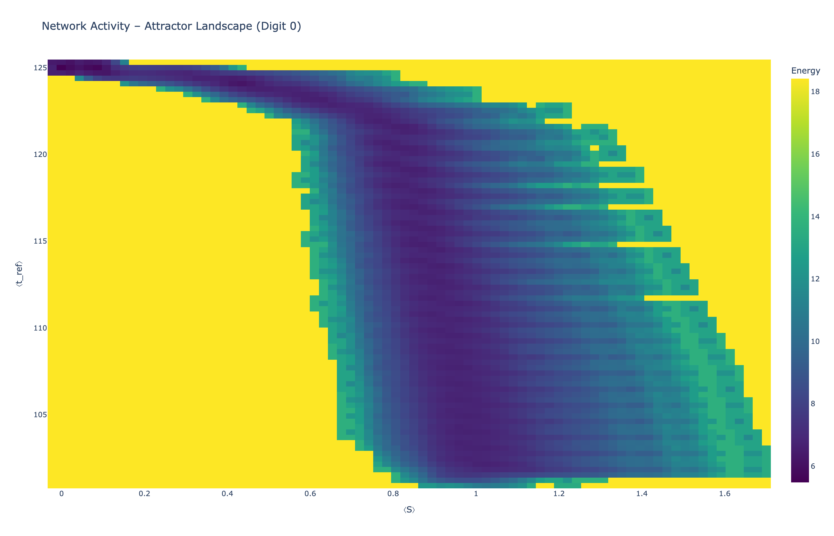
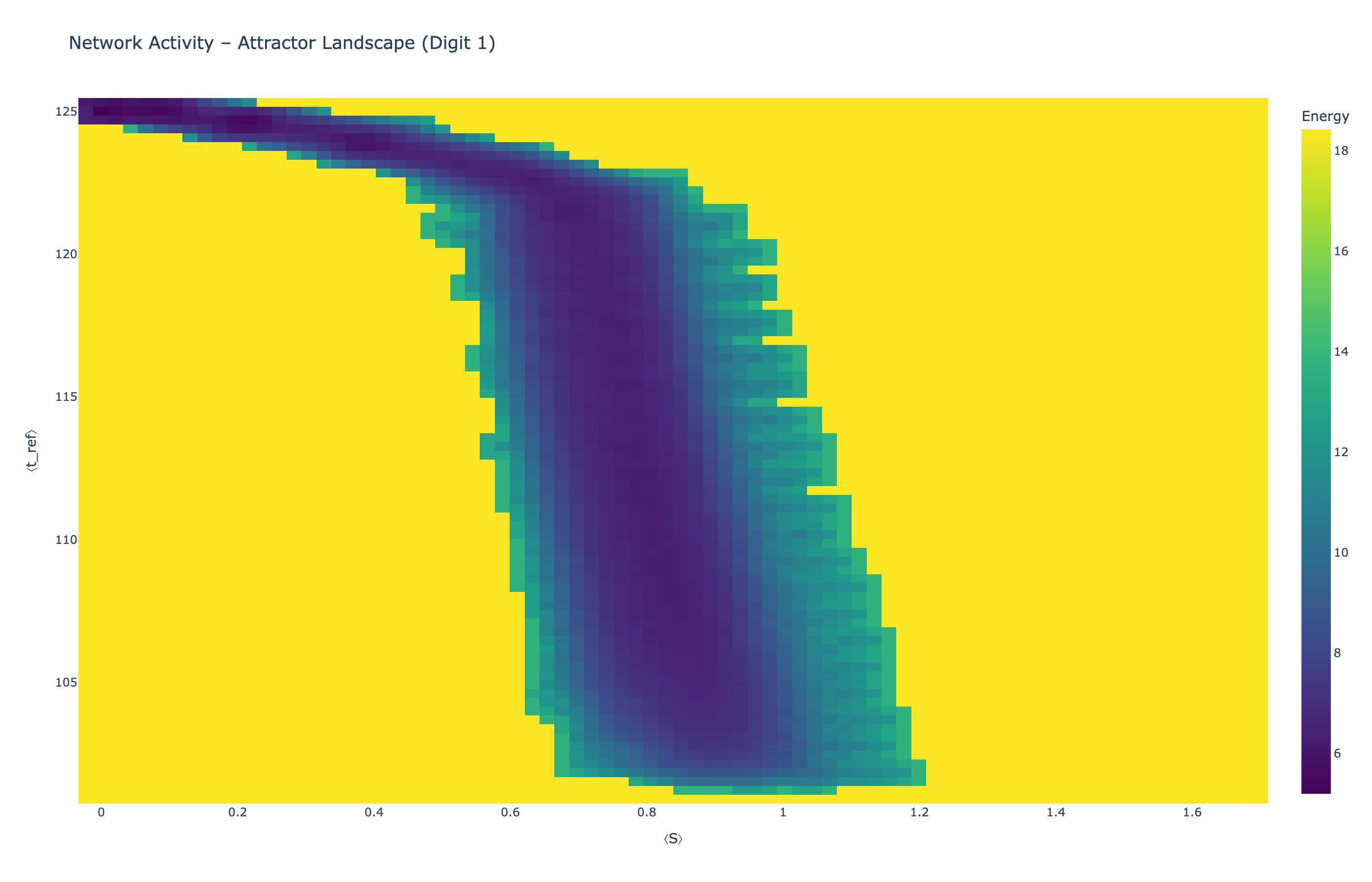
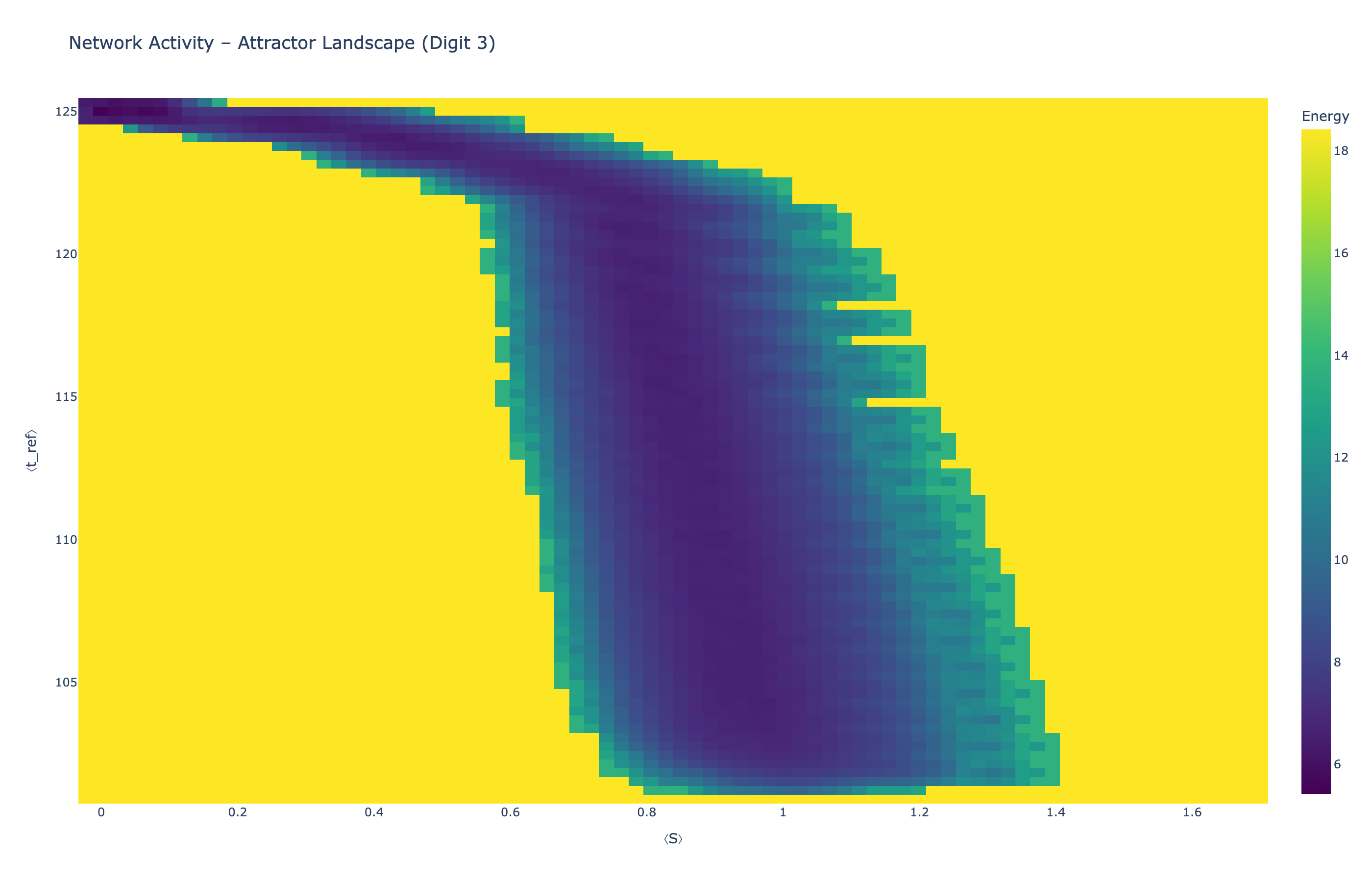
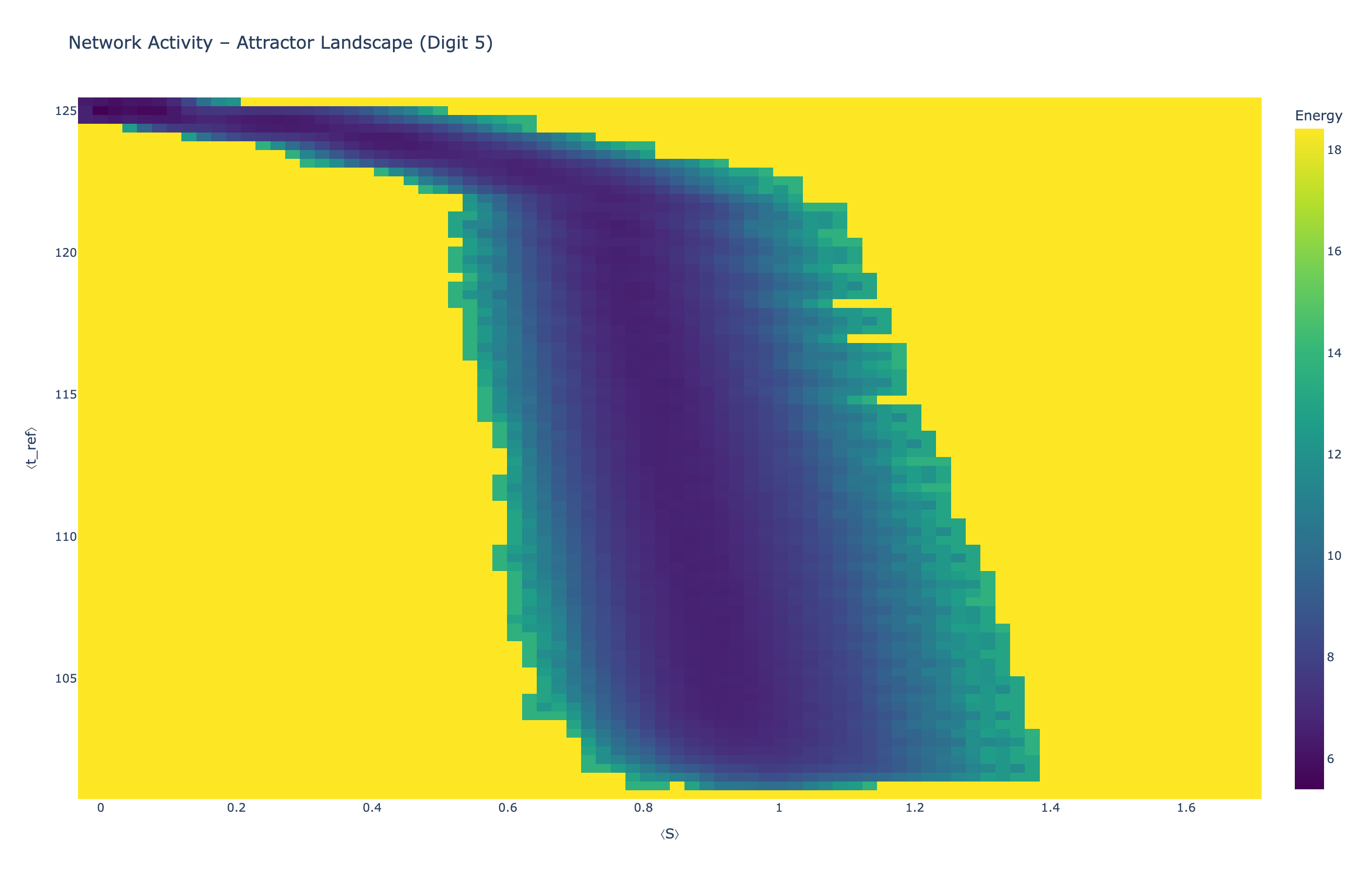
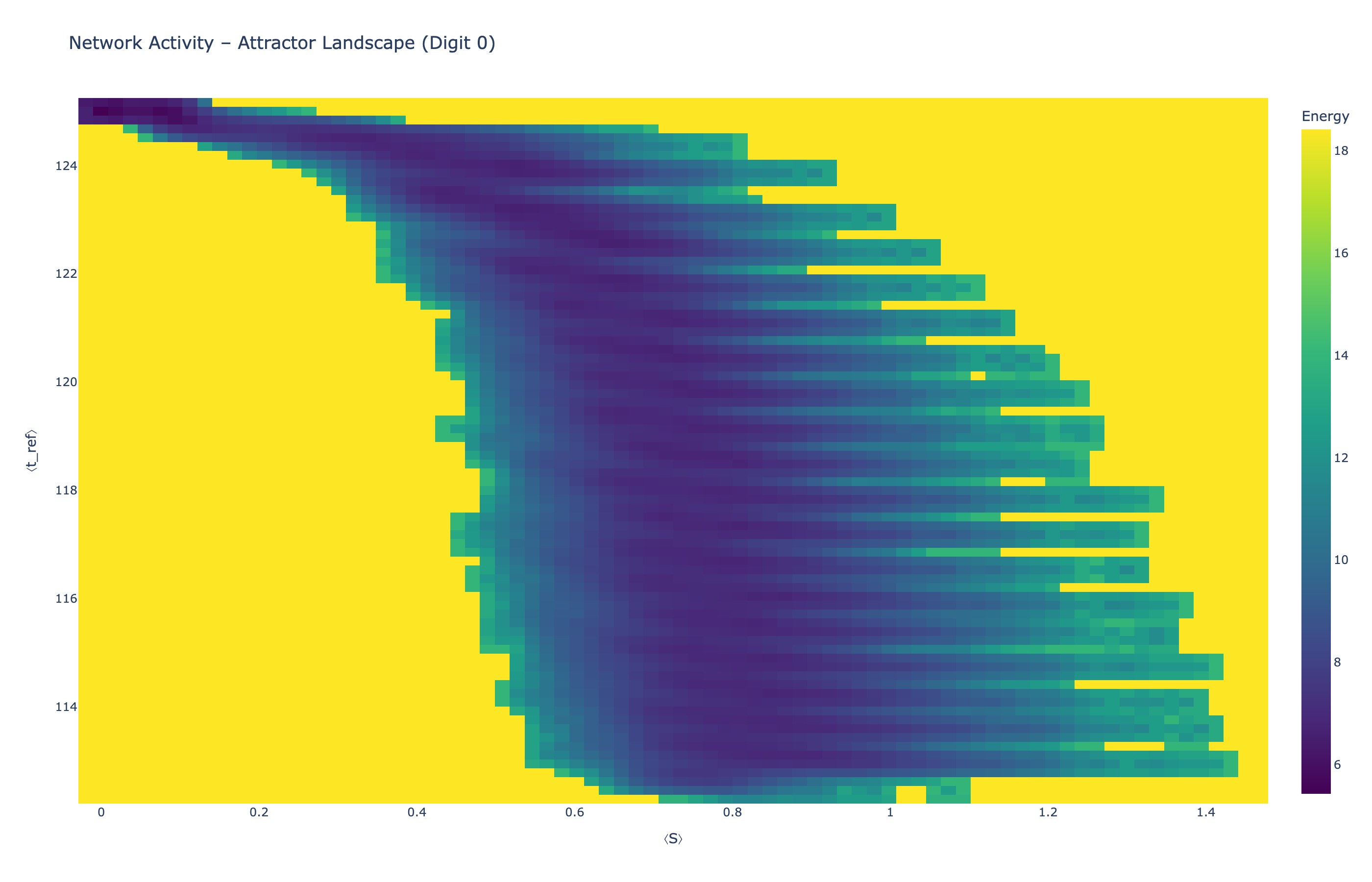
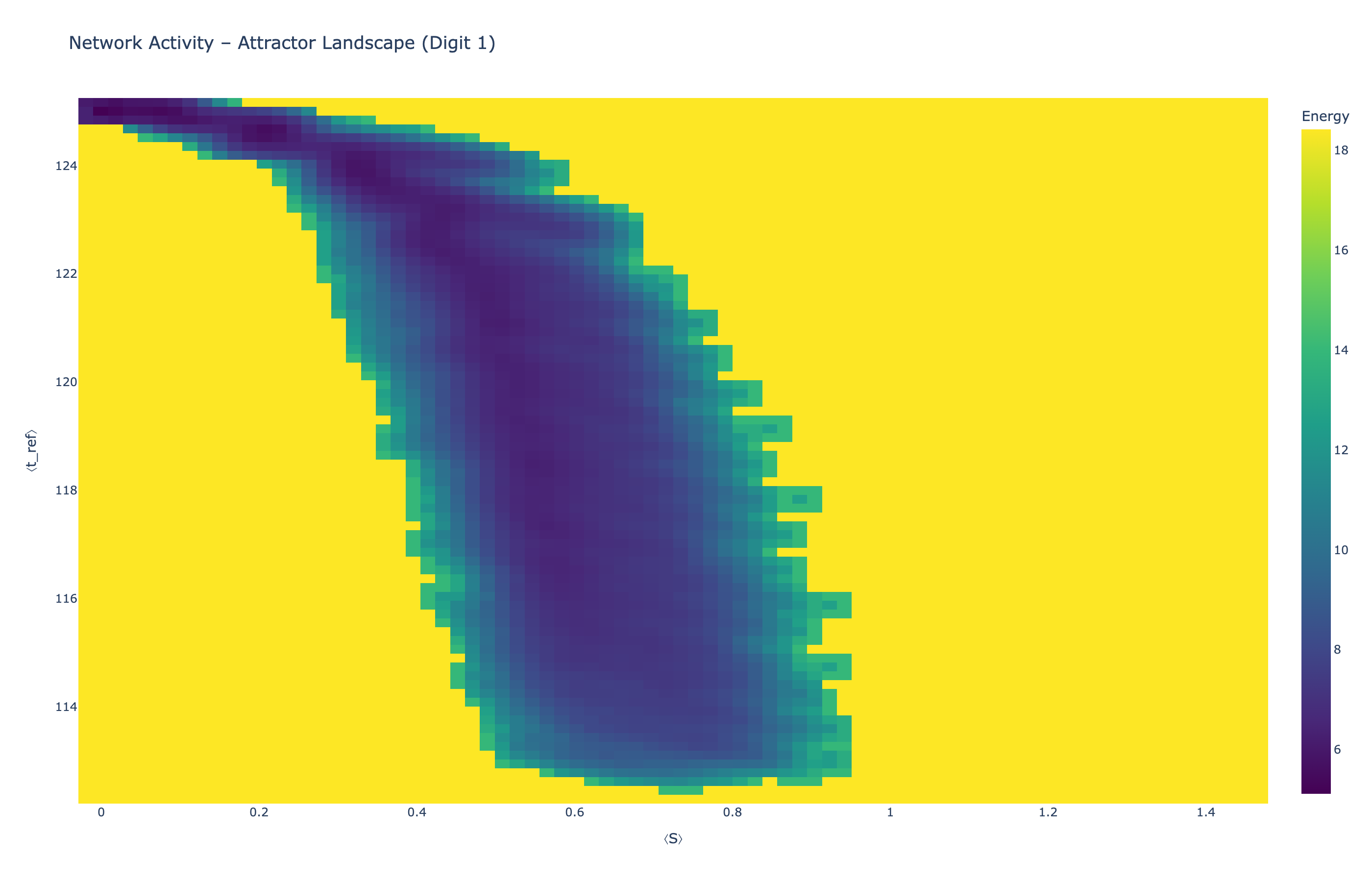
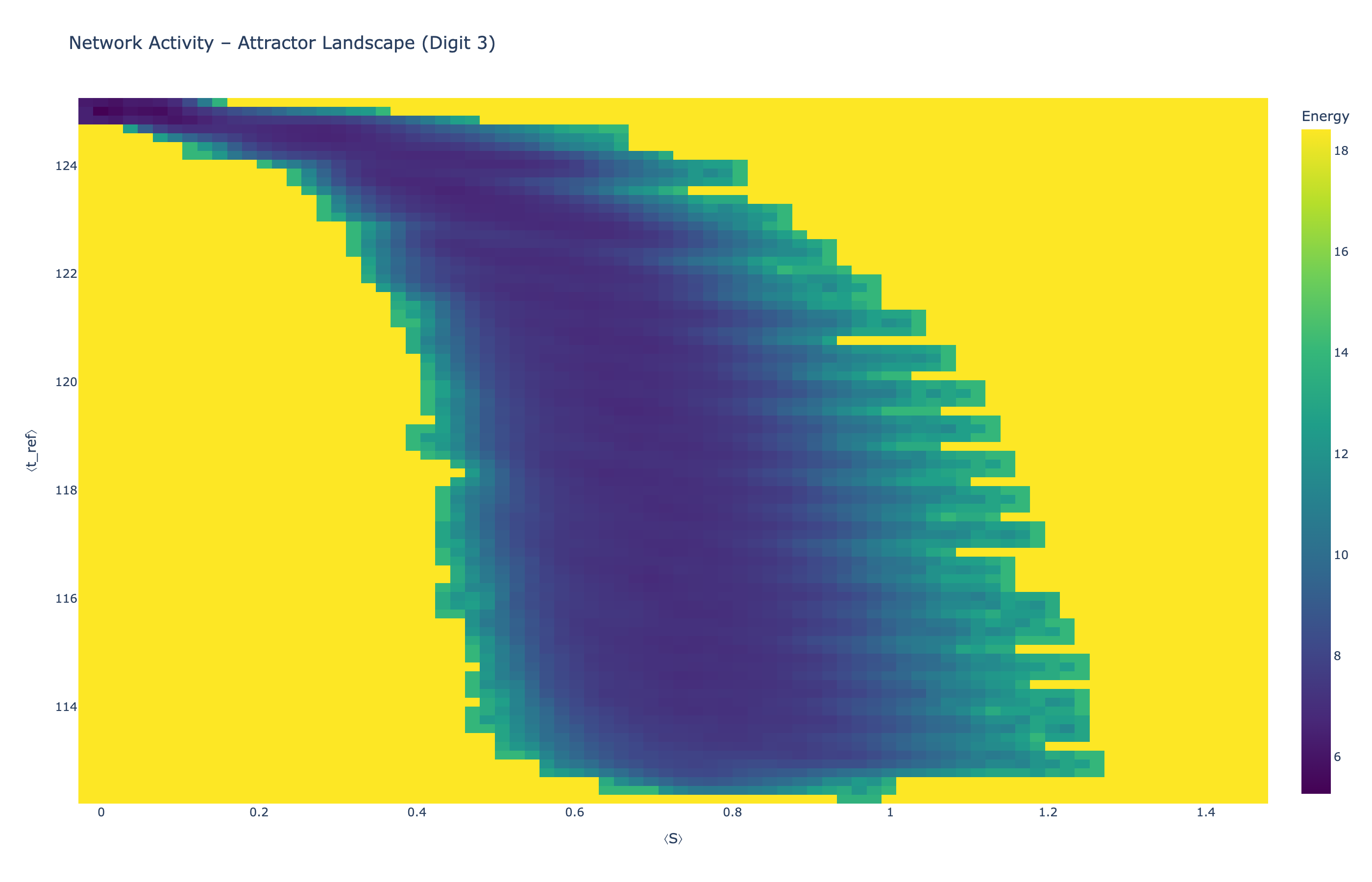
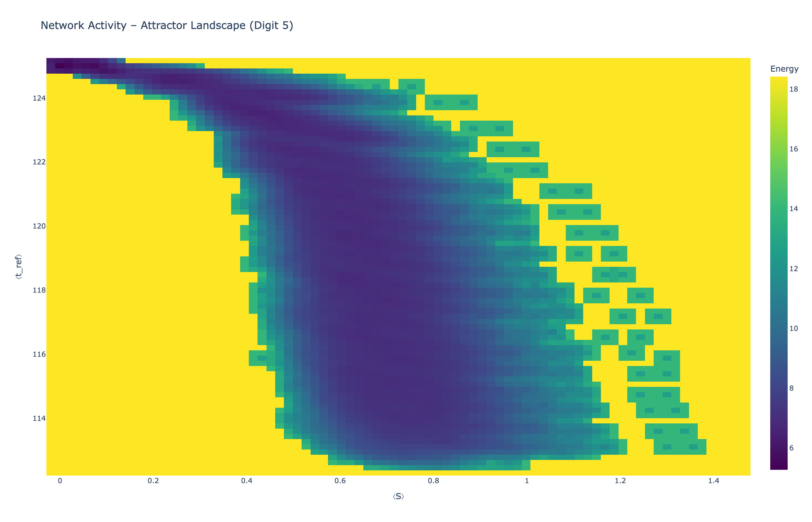
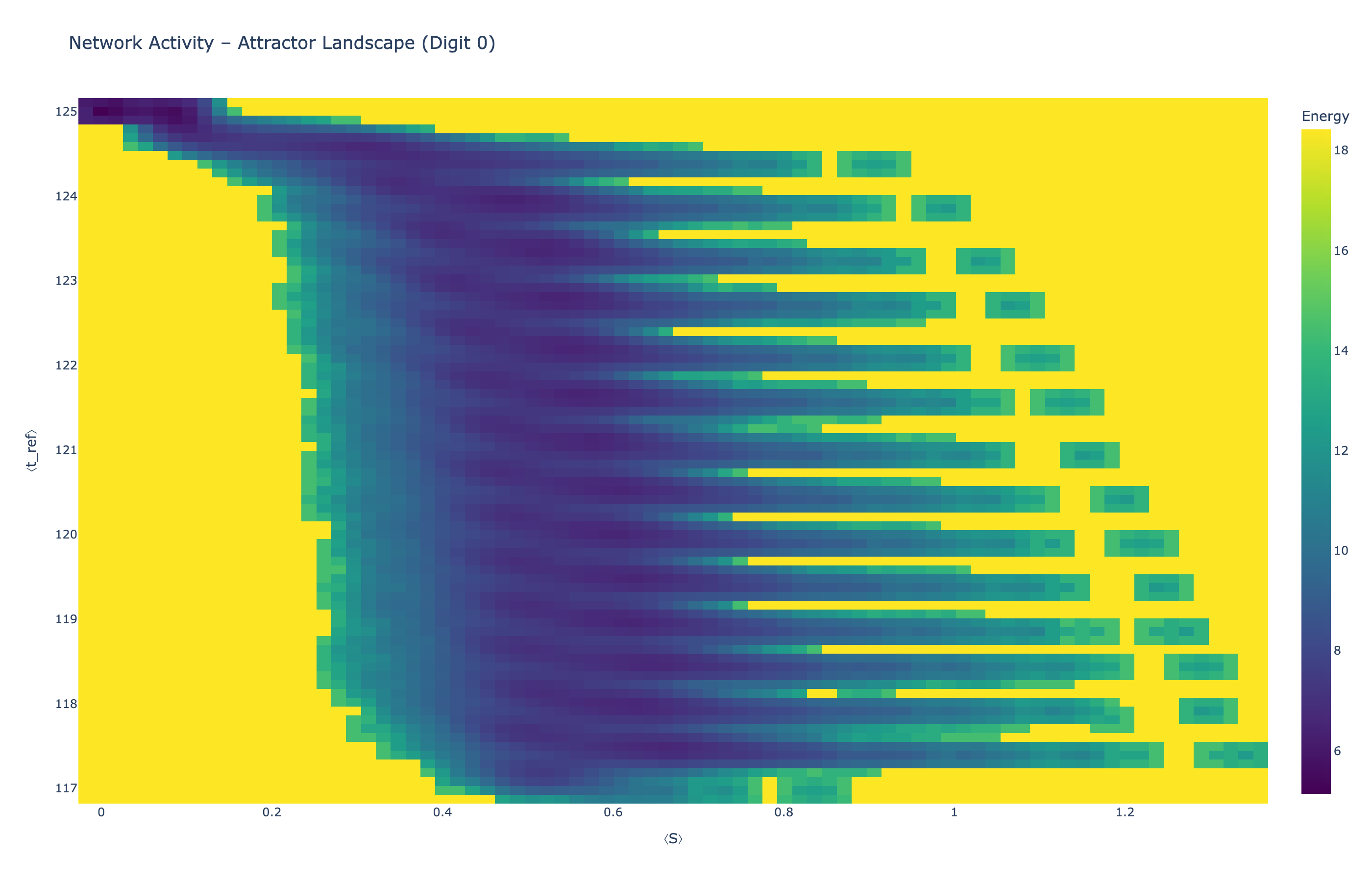
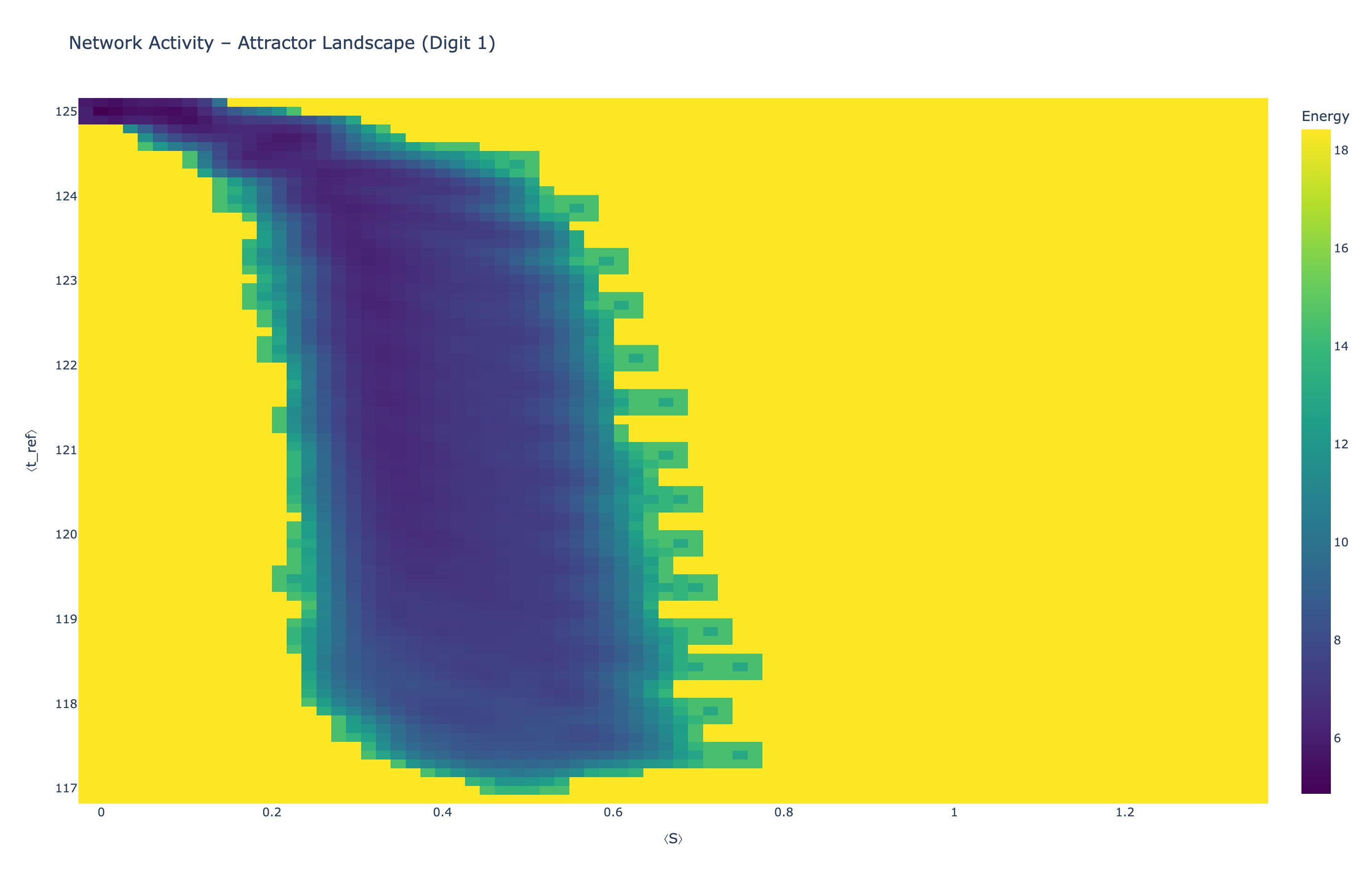
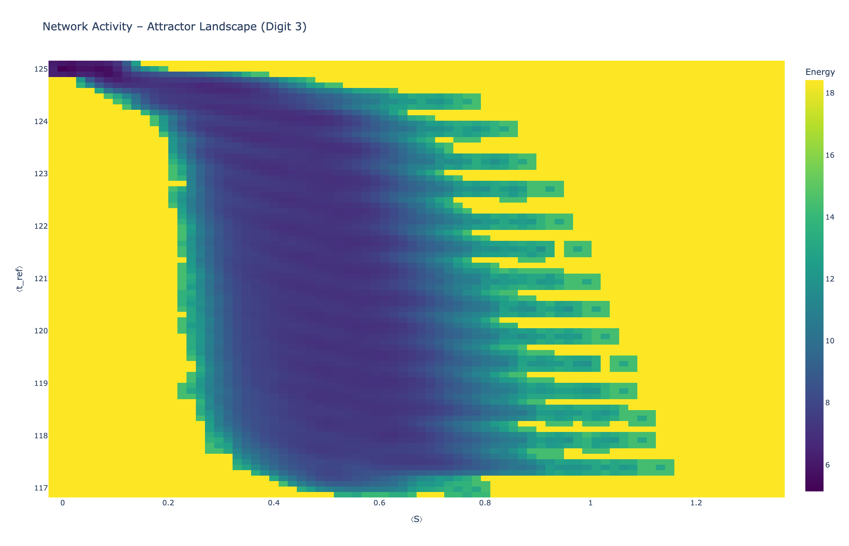
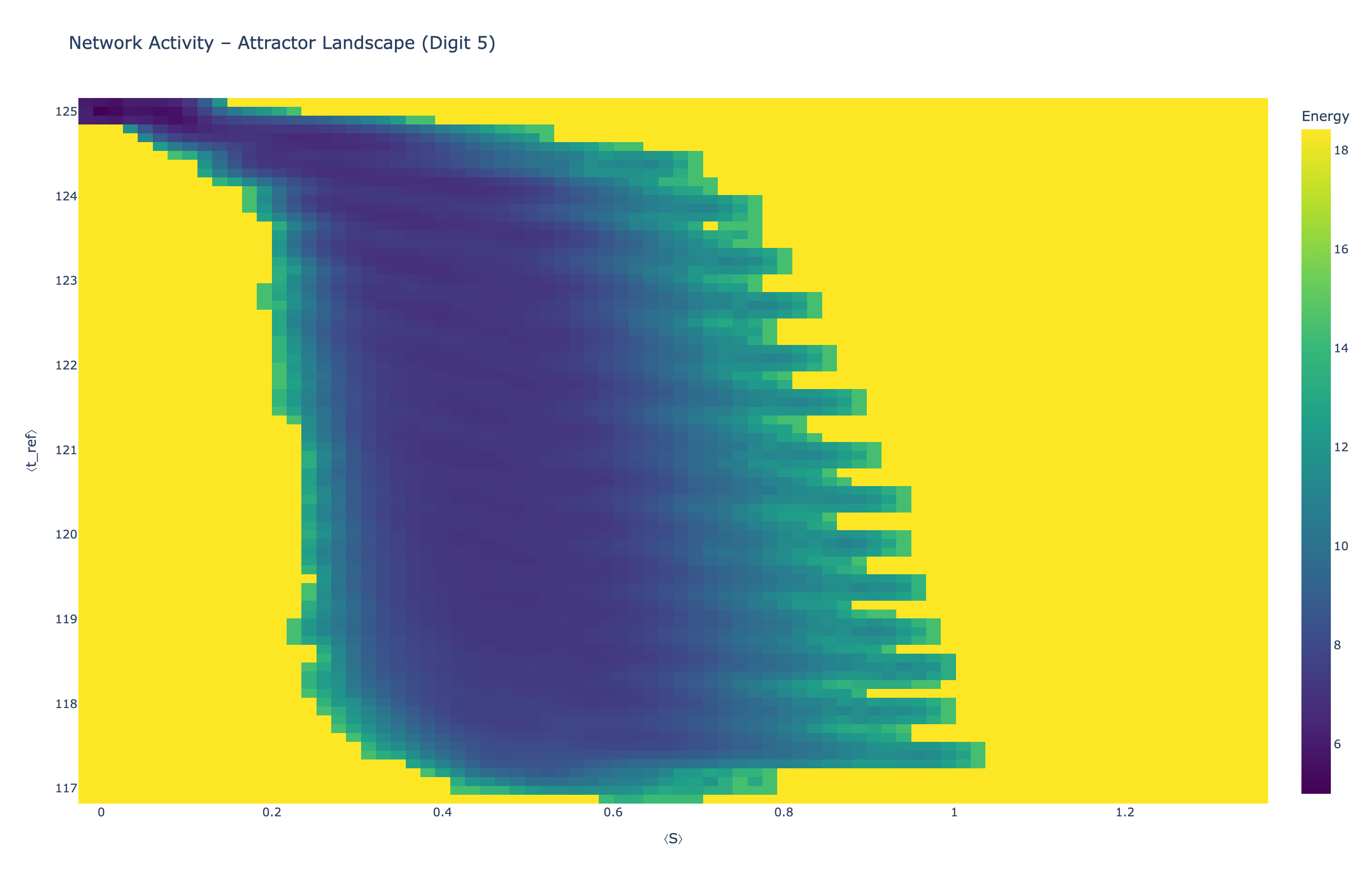
4.5 Attractor Landscapes
We analyzed network state dynamics in (⟨S⟩, ⟨t_ref⟩) space, revealing digit-specific topographies. The table below shows the full comparison across sparsity levels:
| Sparsity | Digit 0 | Digit 1 | Digit 3 | Digit 5 |
|---|---|---|---|---|
| Dense (100%) |
|
|
|
|
| Sparse (50%) |
|
|
|
|
| Sparse (25%) |
|
|
|
|
Figure 5: Attractor landscapes in (⟨S⟩, ⟨t_ref⟩) state space for different digit classes across density levels.
Interactive Attractor Landscapes (25% Sparse Network)
Each panel shows the energy landscape (KDE-smoothed density) for a different digit class. Dark blue regions indicate the network's preferred states (low energy basins); yellow regions represent rarely-visited configurations. Digit 1 exhibits a compact, centered attractor, while Digit 0 shows extended horizontal structure with multiple striations.
These distinct landscape geometries support the processual representation hypothesis: digits are encoded as characteristic dynamical regimes rather than static weight patterns. The network does not store 'digit 0' as a weight pattern but rather as the capacity to enter a specific oscillatory state.
5. Ablation Study: Validating Temporal Dimensionality Expansion
5.1 Rationale
To test whether the coupled multiplicative-homeostatic dynamics are necessary for learning complex temporal patterns, we systematically ablated individual mechanisms. If temporal dimensionality expansion is indeed the core innovation, removing multi-scale integration should cause collapse on complex patterns while sparing simple patterns.
5.2 Methods
We trained seven network configurations on MNIST (1000 samples/digit):
- Baseline: Full PAULA (all mechanisms active)
- Frozen t_ref: Adaptive refractory disabled (fixed at initial value)
- Frozen weights: Synaptic plasticity disabled (random initialization frozen)
- Frozen thresholds: Excitability adaptation disabled
- No retrograde: Presynaptic learning disabled
- No STDP: Directional learning disabled (LTP-only)
- All ablations: All above ablated together
We measured:
- Performance: Top-1 and Top-3 accuracy
- Variance: Per-digit performance variance (stability metric)
- Decision time: Ticks to first correct answer
5.3 Results
Overall Performance
| Configuration | Top-1 Acc | Top-3 Acc | Variance | Decision Time |
|---|---|---|---|---|
| Baseline | 84.3% | 95.6% | 53.82 | 32.1 ticks |
| No retrograde | 84.1% | 95.1% | 71.13 | 42.3 ticks |
| Frozen thresholds | 83.7% | 94.1% | 72.53 | 47.1 ticks |
| Frozen weights | 83.3% | 95.0% | 42.77 | 19.6 ticks |
| No STDP | 82.4% | 95.5% | 76.70 | 28.6 ticks |
| All ablations | 82.2% | 95.1% | 110.05 | 47.1 ticks |
| Frozen t_ref | 80.4% | 94.8% | 250.22 | 46.0 ticks |
Removing adaptive t_ref caused the largest performance loss (-3.9%) and variance explosion (+365%).
Variance Stability Analysis
Variance measures attractor stability: low variance indicates consistent performance across patterns; high variance indicates chaotic, unreliable dynamics.
The variance pattern reveals distinct attractor regimes across configurations. The baseline system maintains moderate variance (53.82), indicating stable learned attractors that generalize across patterns. Networks with frozen weights show even lower variance (42.77) but represent stable random attractors without meaningful learning. Most strikingly, removing adaptive t_ref causes variance explosion to 250.22, indicating complete absence of stable attractors.
The 4.6× variance increase when homeostatic regulation is removed demonstrates that multi-scale projection is essential for attractor stability. Without it, multiplicative learning creates chaotic dynamics that prevent any stable states from forming.
Pattern Complexity Analysis
We analyzed accuracy change by digit complexity:
| Digit | Complexity | Baseline | Frozen t_ref | Decrease in Accuracy |
|---|---|---|---|---|
| 1 | Simple (vertical line) | 97.6% | 99.2% | +1.6% |
| 0 | Simple (single loop) | 94.1% | 94.1% | 0.0% |
| 8 | Complex (loop-connector-loop) | 74.2% | 48.3% | -25.8% |
| 9 | Complex (loop-stem) | 77.7% | 52.1% | -25.5% |
Thinking Time Requirements
The percentage of samples requiring extended deliberation (>50 ticks):
| Digit | Baseline | Frozen t_ref | Interpretation |
|---|---|---|---|
| 1 | 3.2% | 0.8% | Simple = fast decisions |
| 8 | 62.9% | 97.8% | Complex = needs multi-scale |
Without adaptive t_ref, 98% of complex patterns require extended processing (vs. 63% with multi-scale), a 35-point increase demonstrating that unstable attractors significantly slow recall.
5.4 Discussion
The ablation results validate three key hypotheses:
1. Multiplicative weights create exploratory variance
Frozen weights have lowest variance (42.77) because random
initialization is more balanced than learned multiplicative weights.
Learning intentionally creates variance to make temporal structure
explicit. This amplification requires gain control (adaptive t_ref)
to prevent runaway.
2. Adaptive t_ref enables multi-scale projection
Not merely "compensating for instability" but providing the
projection mechanism itself. Creates heterogeneous temporal windows:
short for fast features, long for global context. Enables linear
separability of temporally ambiguous patterns.
3. Expansion degree self-organizes based on signal
statistics
Simple patterns (low variance): Single scale sufficient, close to 0%
loss without expansion.
Complex patterns (high variance): Multi-scale essential, -25%
collapse without expansion.
System automatically adjusts: high-variance signals provoke high
firing rates, causing short t_ref that create selective windows.
Implications: Why Distributed Robustness Is Expected
Individual mechanism removals cost little (1.9% for STDP, 0.2% for retrograde signaling) because in a tightly coupled system, remaining components dynamically compensate when one is disabled. This compensation is not redundancy; it is integration. The correct test of mechanism necessity is total ablation, which removes the compensatory network itself. All-ablation variance (110.05) confirms that the mechanisms collectively produce stability that no proper subset can sustain: the full PAULA system (variance 53.82) is qualitatively different from the all-ablation system (variance 110.05), which in turn is qualitatively different from frozen t_ref alone (variance 250.22). Distributed robustness is the expected signature of an integrated system.
6. Qualitative Observations on Homeostatic Stability
While standard classification operates effectively within short timeframes (e.g., 240 ticks per pattern), we conducted extended observational runs to understand the long-term thermodynamic behavior of the topologies, comparing sparse and dense architectures.
Limit Cycle Attractors vs Chaotic Fluctuations
Rather than tracking quantitative classification metrics over these extended timescales, we observed the internal phase-space trajectory of the plasticity gate (\(t_{ref}\)). In the sparse configurations, the \(t_{ref}\) variable naturally settled into a stable sinusoidal oscillation—a limit cycle attractor.
Phenomenological Observation
The sparse network demonstrates sustainable homeostatic breathing. Conversely, the dense network exhibited chaotic, irregular \(t_{ref}\) fluctuations. Extending the dense network simulation to prolonged intervals did not resolve this instability.
Key Insight
This qualitative observation suggests that beyond a certain density threshold, internal signal interference prevents the network from finding a stable thermodynamic resting state under local homeostatic regulation. This validates that sparse connectivity is beneficial for dynamical stability and temporal coherence in systems relying on local gain control.
This directly parallels biological cortical development. Early postnatal cortex exhibits excessive synaptic density, which undergoes activity-dependent pruning during critical periods. Our results suggest this developmental trajectory is a necessary path to stable neural dynamics.
7. Discussion
7.1 Temporal Dimensionality Expansion as Core Mechanism
The ablation results reveal that PAULA's primary innovation is the coupled dynamics of its mechanisms implementing temporal dimensionality expansion. This reframes our understanding of how bio-inspired SNNs learn temporal patterns.
Traditional interpretations view multiplicative weight updates as problematic, creating instability that requires homeostatic compensation. From this perspective, adaptive mechanisms seem like "nice to have" improvements that add modest performance gains of only 2-3%.
Our ablation results fundamentally challenge this view. Multiplicative weights are not a bug requiring compensation; they are an intentional variance amplifier. By scaling updates proportionally to current weight (Δw ∝ w), they create divergent dynamics where different neurons develop distinct firing rates. This divergence acts as exploration pressure that forces neurons to specialize.
Similarly, adaptive refractory periods convert exploration into productive specialization. High-firing neurons, having developed large weights through high-variance patterns, develop short refractory periods that make them selective to fast temporal features. Low-firing neurons develop long refractory periods that make them integrative of slow global structure. Together, this heterogeneity creates the multi-scale representation essential for complex pattern learning.
Together, these mechanisms appear to implement a temporal kernel trick. The system begins with compressed temporal patterns that are temporally ambiguous. Multiplicative weights amplify variance across neurons, creating divergent firing rates where different neurons develop different response properties. Adaptive refractory periods then project these signals into multi-scale temporal windows, creating heterogeneous temporal integration that captures both fast transitions and slow global structure. The result is a high-dimensional multi-scale representation where temporally ambiguous patterns become linearly separable.
This process mirrors classical kernel methods, which map inputs to higher-dimensional spaces to enable linear separation. However, while kernel methods use fixed mappings, PAULA's multi-scale projection self-organizes based on input statistics through variance-driven adaptation, automatically adjusting expansion degree to match pattern complexity.
These results carry significant biological implications. Cortical heterogeneity (neurons with different temporal properties, from fast-spiking interneurons to regular-spiking pyramidal cells) is fundamentally functional. This diversity enables multi-scale temporal processing necessary for complex pattern recognition. The brain creates multiple parallel temporal views of the same input, each emphasizing different timescales, allowing complex temporal patterns to be disentangled through integration across scales.
7.2 The Processual Representation Hypothesis
This section presents a key theoretical contribution of this work: a reconceptualization of what it means for a neural system to represent something. Standard accounts treat representation as a state of weights. PAULA's dynamics suggest a different perspective.
The finding that different digits drive the network into different dynamical regimes supports a processual view of representation. The network stores 'digit 0' not as a pattern in weight space, but as the capacity to enter an oscillatory state characterized by 15-tick periodicity and growing variance amplitude. Classification is re-enactment: the network recreates the dynamics it previously associated with that input. This aligns with enactivist cognitive science and predictive coding frameworks, while providing computational instantiation with measurable state variables.
This processual view suggests rethinking how we design learning systems. Rather than asking 'what weights represent X?', we should ask 'what state corresponds to X?' and 'how does the system transition between states?'
- Memory becomes the landscape of attractors, not a database of patterns
- Learning becomes niche construction in state space, not gradient descent in weight space
- Forgetting becomes inability to access attractors, not weight overwriting, suggesting solutions to catastrophic forgetting through state-space partitioning
Extending this approach toward artificial general intelligence requires augmenting perceptual classification with goal-directed behavior and self-monitoring. Our broader research program proposes supervisory networks that observe the system's own state dynamics, creating meta-level representations. These supervisors could detect anomalies, specifically states that do not match expectations, regulate homeostatic setpoints based on task demands, and potentially give rise to self-awareness through recursive observation of observation. The current work establishes that state-based representations are computationally viable; future work must demonstrate they support flexible, goal-directed cognition.
7.3 Architectural Priors and the Variance Constraint
Our experiments reveal a critical relationship between network topology and input statistics: while the PAULA neuron is entirely modality-agnostic and will dynamically model any continuous input stream, the network's macroscopic ability to separate temporal trajectories relies on spatial variance. With flattened RGB inputs in a dense Multilayer Perceptron (MLP) topology (e.g., CIFAR-10), performance is limited due to lower pixel-level variance compared to the high-contrast edges characteristic of MNIST.
This is a strict requirement for topological alignment. This architectural variance constraint yields a falsifiable theoretical prediction: a flat PAULA topology will succeed on inputs with high intrinsic variance, but will struggle to resolve low-variance, dense sensory streams without hierarchical feature extraction. When arranged in a spatial hierarchy featuring the appropriate inductive priors, the model successfully projects low-variance density into highly separable temporal domains, as demonstrated in our 96.55% convolutional result.
7.4 Interpretability Challenges
An interesting paradox emerged from our analysis: functional specialization is evident through population analysis but resists traditional single-unit ablation studies. This actually validates the biological realism of the substrate. Like natural neural systems, our model exhibits graceful degradation (Result 3) and distributed representation, requiring neuroscience-appropriate analysis methods rather than standard ML interpretability techniques.
7.5 Global Context for Local Learning
While this work validates the core predictive learning and homeostatic metaplasticity mechanisms (Kuśmierz et al., 2017), the model's neuromodulation framework (\(\vec{M}(t)\) dynamics) enables future investigation of context-dependent learning, attention-like modulation, and task-switching, capabilities essential for embodied agents in dynamic environments.
Specifically, the model explicitly supports arbitrary neuromodulator types which can be seamlessly integrated in any internal process of a single neuron, from regulating the postsynaptic integration to affecting the decay factors of traveling signals and more.
7.6 Synaptic Weight Dynamics
Our validation establishes that the local learning mechanisms produce functional networks, but characterizing the emergent weight structures, learning trajectories, and the specific contribution of retrograde error correction requires dedicated analysis. Such investigation would reveal how the network's internal representations develop over training and could inform optimal initialization strategies.
Crucially, our model establishes that contrary to traditional AI systems, synaptic weights are not the only storage for information in neural networks. When the complex structure of a biological neuron is respected, it allows for a different type of information storage which does not rely solely on synaptic weight distribution or spike trains in SNNs. The dimensionality reduction power of a single computational unit (784 synapses reduced down to membrane potential and plasticity window with ~40% of preserved information) strongly supports that internal neuron dynamics and structure play a major role in bio-plausible computational systems (Ding et al., 2025; Intrator & Cooper, 1992).
The single neuron's capacity for intelligent dimensionality reduction suggests that biological neurons may function as nonlinear embedding units, projecting high-dimensional sensory input onto low-dimensional manifolds that preserve task-relevant structure. This spatiotemporal dimensionality reduction parallels recent work on nonlinear transforms for compression, which demonstrated that neural representations can achieve massive compression by transforming data into domains where redundancy is more efficiently encoded.
7.7 Sparsity Scaling Law and Network Architecture
The sparsity scaling law suggests a broader architectural principle: representation quality requires constraints on information flow. In dense networks, these constraints come from depth (vertical segregation); in shallow networks, they must come from sparsity (horizontal segregation). This explains both the success of deep learning architectures and the efficiency of biological sparse cortical networks, which employ both strategies simultaneously.
7.8 Architecture Search via Homeostatic Stability
Our long-term dynamics findings suggest a novel principle for neural architecture design: architectures should be optimized for homeostatic stability rather than immediate task performance. This criterion, selecting networks that achieve dynamical equilibrium within feasible timescales, provides a biologically-grounded alternative to gradient-based neural architecture search (NAS) approaches.
Traditional NAS methods optimize architectures through task-specific performance metrics, requiring extensive labeled data and computational resources for evaluating each candidate. In contrast, stability-based selection requires only observation of intrinsic dynamics under unlabeled input, as homeostatic convergence is a property of the network's response to input statistics, not task labels. An architecture that fails to stabilize, as we observed with dense networks, cannot form reliable internal representations regardless of task, filtering it out before expensive task evaluation.
The biological plausibility of this approach is evident in cortical development. Early cortex exhibits random, excessive connectivity, which undergoes activity-dependent refinement through synaptic pruning, homeostatic scaling, and inhibitory tuning. These mechanisms do not optimize for specific tasks (the infant does not yet know what tasks it will encounter) but rather establish stable, adaptive computational substrates that can subsequently learn diverse skills.
The observed scaling of stabilization effort with input dimensionality provides qualitative intuition for architecture design:
- Small inputs (e.g., MNIST): phase-space stabilization is readily observable in reasonable timeframes.
- Moderate inputs (e.g., CIFAR-10): extended observation reveals longer trajectories before limit cycles emerge.
- Large inputs (e.g., ImageNet): monolithic architectures likely face extreme stabilization demands, suggesting the need for hierarchical processing where lower layers stabilize on local receptive fields before deeper layers integrate globally.
7.9 Biological Parallels: Development, Pruning, and Stability
Our finding that sparse networks achieve stability while dense networks remain perpetually unstable provides computational support for a long-standing puzzle in neurodevelopment: why does cortex initially overproduce synapses, only to eliminate 40-60% during postnatal critical periods? Traditional explanations emphasize metabolic efficiency or Darwinian selection of "useful" connections. Our results suggest a complementary mechanism: pruning enables dynamical stability under local homeostatic regulation.
In early postnatal cortex, synaptic density peaks at approximately twice the adult level, then undergoes activity-dependent pruning during critical periods. This developmental trajectory parallels our findings: dense initial connectivity (analogous to 100% networks) creates unstable dynamics where homeostatic mechanisms cannot converge. Pruning to sparse adult levels (analogous to 25% networks) enables stabilization. The brain may not "know" which specific connections to eliminate; instead, activity-dependent mechanisms remove connections until the network enters a stable dynamical regime where homeostatic regulation can converge.
This interpretation is consistent with experimental observations that synaptic pruning is triggered by neural activity patterns and regulated by homeostatic mechanisms. Networks with excessive connectivity show heightened excitability and instability. Pruning reduces this instability, enabling refinement of functional circuits. Disruptions to this process, as occur in neurodevelopmental disorders where pruning is impaired, result in networks with persistent instability, potentially underlying the sensory hypersensitivity and information processing deficits observed in autism spectrum disorders and schizophrenia.
The cross-layer functional organization that emerges in our stabilized sparse networks further parallels cortical development. Orientation columns in V1, for instance, develop through spontaneous activity-driven self-organization before visual experience, with neurons across layers coordinating based on response properties rather than anatomical proximity. Our model reproduces this emergent organization through purely local homeostatic mechanisms, supporting theories that cortical columns arise from stabilization of initially random connectivity under homeostatic constraints.
Cortical Multi-Scale Processing: The ablation results provide a functional explanation for cortical neuronal diversity. Fast-spiking interneurons (short integration windows) and regular-spiking pyramidal neurons (long integration windows) may constitute a biological implementation of temporal dimensionality expansion. Our finding that complex patterns collapse 25% without multi-scale integration proves this diversity is a computational necessity.
The 90-150 tick range in PAULA aligns with cortical temporal dynamics. The slowdown in recall without heterogeneous t_ref (98% of complex patterns requiring extended processing vs. 63% with multi-scale) mirrors the speed-accuracy tradeoffs observed in human perceptual decisions. This positions PAULA as a computational framework for investigating principles of neural development and multi-scale temporal processing.
7.10 Resistance to Catastrophic Forgetting
A persistent challenge in modern Artificial Neural Networks (ANNs) is catastrophic forgetting, where learning new information rapidly overwrites previously learned representations because backpropagation fundamentally relies on global scalar updates to synaptic weights.
In contrast, PAULA provides a natural, physical resistance to catastrophic forgetting. Because the architecture relies on physical temporal delays and localized attractors (limit cycles), memories are structurally bound to specific topological basins in the network's state space. This structural binding ensures that novel sensory data cannot instantly overwrite established temporal representations, offering a biologically-plausible mechanism for continual learning.
8. Limitations and Future Work
While PAULA demonstrates significant temporal dimensionality expansion, the experimental validation presented in this work utilizes static initializations for specific temporal parameters to isolate the effects of adaptive \(t_{ref}\). Consequently, the current proof-of-concept pipeline requires careful initial tuning of the \(\lambda\) integration constants to match expected stimulus lengths, and relies on fixed, randomly initialized spatial delays (\(d\)) to construct its temporal topology.
We emphasize that these static variables are artifacts of the current experimental initialization, rather than theoretical limitations of the ALERM framework. Because the architecture supports an arbitrary number of concurrent neuromodulators, future work may implement dynamic meta-plasticity rules where \(\lambda\) is continuously regulated by dedicated neuromodulatory state vectors, allowing individual neurons to autonomously tune their integration windows to shifting input frequencies. Similarly, future iterations will explore dynamic routing and adaptive delays (\(d(t)\)), systematically quantifying the cross-seed topological variance currently observed in static initializations.
9. Conclusion
This work makes three contributions:
- A formal model of homeostatic metaplasticity integrating dynamic learning windows with vector synapses and local predictive learning
- Empirical validation suggesting this mechanism enables competitive performance (86.8% MNIST) with purely local rules
- Discovery that different input classes drive networks into distinct dynamical regimes with characteristic temporal signatures
A network of these adaptive neurons is a self-organizing system whose primary emergent function is the construction of a robust internal model. The model's Hebbian learning rule naturally gives rise to cell assemblies: interconnected groups of neurons that represent stable concepts, objects, and causal relationships in the environment. Information is therefore not stored in any single neuron but is encoded in the distributed patterns of activity across these populations.
A critical challenge in any plastic network is maintaining stability. This model addresses the problem from the bottom up through homeostatic plasticity. Each neuron's metaplasticity rule (Kuśmierz et al., 2017), which adjusts its learning window based on its average firing rate, provides a powerful local stabilizing force. If a circuit becomes over-excited, its constituent neurons automatically reduce their learning sensitivity, preventing runaway potentiation and ensuring the network's internal representations remain stable.
This model's architecture provides a framework for addressing several key open problems across multiple disciplines:
In AI and machine learning, it offers a plausible, local alternative to the credit assignment problem solved by backpropagation, using a retrograde signaling loop to provide targeted feedback. It addresses continual learning and catastrophic forgetting through its inherent homeostatic plasticity, and its sparse, event-driven nature as a Spiking Neural Network (SNN) makes it a candidate for highly energy-efficient computation.
In neuroscience, the model provides a unified mathematical framework for exploring how different forms of plasticity, Hebbian, homeostatic, and neuromodulatory, can coexist and interact. Its graph-based structure provides a testable platform for investigating the role of dendritic computation, and its use of sensitivity vectors offers a quantitative hypothesis for the function of neuromodulatory diversity.
In cognitive science and philosophy, the model provides a plausible mechanistic substrate for several theories. The temporal synchronization of its neurons can address the "binding problem" of perception. Its self-organizing nature aligns with theories of internal representation where the brain builds a predictive model of its environment. And its capacity for information integration, global coordination, and self-reflection aligns with key principles of scientific theories of consciousness, such as Integrated Information Theory (IIT) and Global Workspace Theory (GWT).
These results demonstrate that local learning with homeostatic regulation is viable for complex tasks and open paths toward neuromorphic implementations and continual learning systems, bridging the gap towards nonbiological life forms.
Future architectural extensions appear promising. Preliminary exploration of convolutional implementations demonstrated 96.55% MNIST and 87.1% FashionMNIST accuracy on unoptimized first runs, exceeding the classic Diehl & Cook (2015) purely-local benchmark. These results are significant because the convolutional variant uses the same PAULA neuron model and local learning rules as the MLP experiments presented above; only the connectivity topology changes to provide spatial inductive priors. This validates a key ALERM prediction: that the framework's principles are architecture-agnostic and transfer across topologies when appropriate structural priors are provided for the input domain.
Top-3 accuracies of 99.3% (MNIST) and 98.3% (FashionMNIST) indicate that the convolutional PAULA representations are highly discriminative; remaining Top-1 gaps reflect decision confidence rather than perceptual failure. Grayscale CIFAR-10 reaches ~50% accuracy on a 600-neuron network, consistent with the architectural variance constraint discussed in §7.3: low-variance dense inputs require hierarchical feature extraction that flat topologies cannot provide. Together with systematic hyperparameter optimization, these results suggest PAULA's principles extend well beyond the MLP architecture demonstrated here.
10. Related Work
This work builds upon and relates to several important research directions in neuroscience-inspired AI. While the full list of references is below, three specific comparisons highlight PAULA's unique contributions:
- BCM Theory: BCM theory regulates the LTP/LTD threshold (θ_M) via a temporal average of postsynaptic activity -s synaptic-level metaplasticity. PAULA combines this kind of synaptic regulation (through adaptive thresholds on the multiplicative weight update) with neuronal-intrinsic plasticity (Daoudal & Debanne, 2003; Zhang & Linden, 2003): the adaptive refractory period t_ref modulates the cell's integration window and excitability based on its own firing history. Both mechanisms are history-dependent homeostatic regulation; PAULA's contribution is the specific composition of synaptic and intrinsic plasticity, with t_ref operating as a temporal eligibility window in addition to its excitability role.
- Biological Capacity: Jones & Kording (2020) demonstrated that biological dendritic neurons can solve MNIST through compartmentalized spatial computation. Our single PAULA neuron achieves comparable capacity through temporal dimensionality expansion, suggesting spatial dendritic branching and temporal graph delays may be functionally equivalent substrates for single-unit computation.
- Local Learning: While models like DECOLLE utilize local surrogate gradients with fixed learning dynamics, PAULA introduces an adaptive temporal gate ($t_{ref}$) that entirely bypasses the need for surrogate gradient estimations during local weight updates.
Complete Bibliography:
- The Universal Landscape of Human Reasoning (Chen et al., 2025)
- Advancing the Biological Plausibility and Efficacy of Hebbian Convolutional Neural Networks (Nimmo & Mondragón, 2025)
- Objective function formulation of the BCM theory of visual cortical plasticity: Statistical connections, stability conditions (Intrator & Cooper, 1992)
- A Computational Perspective on NeuroAI and Synthetic Biological Intelligence (Patel et al., 2025)
- Neural Brain: A Neuroscience-inspired Framework for Embodied Agents (Liu et al., 2025)
- Continuous Thought Machines (Darlow et al., 2025)
- The Dragon Hatchling: The Missing Link between the Transformer and Models of the Brain (Kosowski et al., 2025)
- Implementing Spiking World Model with Multi-Compartment Neurons for Model-based Reinforcement Learning (Sun et al., 2025)
- An Accurate And Fast Learning Approach In The Biologically Spiking Neural Network (Nazari & Amiri, 2025)
- Training High-Performance Low-Latency Spiking Neural Networks by Differentiation on Spike Representation (Meng et al., 2023)
- Synaptic Plasticity Dynamics for Deep Continuous Local Learning (DECOLLE) (Kaiser et al., 2020)
- Keys to Accurate Feature Extraction Using Residual Spiking Neural Networks (Vicente-Sola et al., 2022)
- Learning with Three Factors: Modulating Hebbian Plasticity with Errors (Kuśmierz et al., 2017)
- Three-Factor Learning in Spiking Neural Networks: An Overview of Methods and Trends from a Machine Learning Perspective (Mazurek et al., 2025)
- Predictive Coding Approximates Backprop along Arbitrary Computation Graphs (Millidge et al., 2020)
- On the Adversarial Robustness of Spiking Neural Networks Trained by Local Learning (Lin & Sengupta, 2025)
- Graph World Model (Feng et al., 2025)
- Advancing Spatio-Temporal Processing in Spiking Neural Networks through Adaptation (Baronig et al., 2025)
- Information-computation trade-offs in non-linear transforms (Ding et al., 2025)
- Brain-inspired Artificial Intelligence: A Comprehensive Review (Ren & Xia, 2024)
- Learning the Plasticity: Plasticity-Driven Learning Framework in Spiking Neural Networks (Shen et al., 2024)
- The neuron as a direct data-driven controller (Moore et al., 2024)
- Hebbian Deep Learning Without Feedback (Journé et al., 2023)
- Biophysical models of intrinsic homeostasis: Firing rates and beyond (Niemeyer et al., 2022)
- Predictive Coding Light (N'dri et al., 2025)
- Can Single Neurons Solve MNIST? The Computational Power of Biological Dendritic Trees (Jones & Kording, 2020)
- STDP-based spiking deep convolutional neural networks for object recognition (Kheradpisheh et al., 2017)
- Sleep-Based Homeostatic Regularization for Stabilizing Spike-Timing-Dependent Plasticity in Recurrent Spiking Neural Networks (Massey et al., 2026)
- Adaptive Synaptic Scaling in Spiking Networks for Continual Learning and Enhanced Robustness (Xu et al., 2025)
- Multi-compartment Neuron and Population Encoding Powered Spiking Neural Network for Deep Distributional Reinforcement Learning (Sun et al., 2025)
- Fast and robust learning in Spiking Feed-forward Neural Networks based on Intrinsic Plasticity mechanism (Zhang et al., 2019)
- TESS: A Scalable Temporally and Spatially Local Learning Rule for Spiking Neural Networks (Apolinario et al., 2025)
- Energy optimization induces predictive-coding properties in a multi-compartment spiking neural network model (Zhang et al., 2025)
- Supervised learning of spatial features with STDP and homeostasis using Spiking Neural Networks on SpiNNaker (Davies et al., 2024)